Jensen’s inequality
What is a convex position?
Any activity that result in unlimited potential upside with a limited quantifiable downside can be called convex.
e.g., Learning, writing a book, research, start-ups and buying derivatives are similar; they are all convex. Risk of failure is high, but the reward one may recieve if successful will be life changing.
Risk and pay-off graph
Assume that we have a pay-off, g, which is a convex function of risk, x, given by f(x)=g.
Let us plot risk, x, in x axis and pay-off, g, in y axis. When we go to the right in the x axis, risk goes on increasing and at one point x2, risk is 100%. We can loose everything deployed. Yet the reward is exponentially high to ignore,1000%!. In the extreme left, x1 , we can deploy the same asset with zero risk to get a modest return of 9%. Let the probability of x1 be p1 and probability of x2 be p2. p1 is extremely likely event and p2 is less likely event, and they can be unrelated. But for simplicity, p1 is around 66% and p2 is around 33% ( assuming that x2 happens when ever market moves more than 10% in either directions in 6 months). The below diagram graphically depicts the above mentioned scenario.
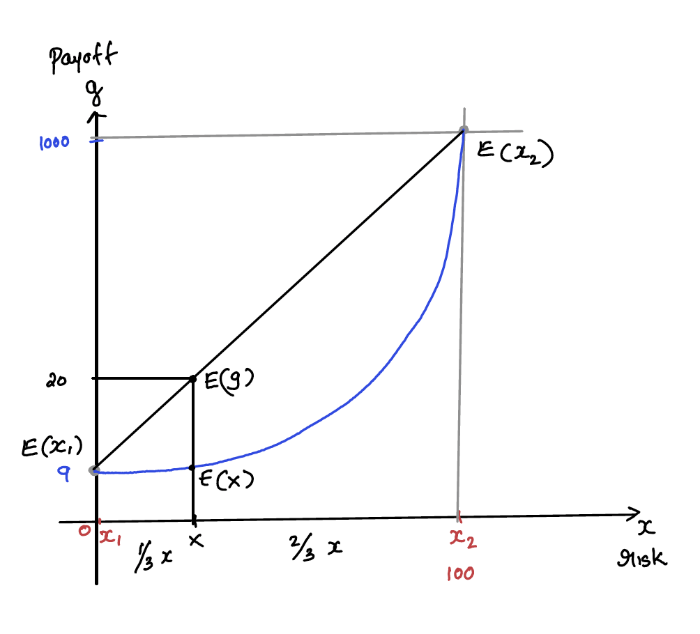
If all assets are deployed at x1, we can generate a return of f(E(x1))=9% with very high probability of success with almost zero risk. On the other hand, if we deploy all the assets at x2, we may generate a mind blowing return of f(E(x2))=1000%, but with a very high probability of 100% capital loss.
Assume we have a combination of x1 and x2. Here, Jensen’s inequality says that expected value of g will always be greater than or equal to the function of the expected value of x, given that the f(x) is convex
\[ E(g) >= f(E(x)) \]
Conclusion
Never put all eggs in one basket of similar risk-pay-off profile.
Our immediate hunch will be to distribute the asset in all possible values of x to get an expected pay-off which is greater than the sum of the individual returns. This is true for a single period return.
Problem with this is, when we invest for multiple periods without rebalancing, the approach neglect the following facts:
the money weighted moral expectation (geometric mean) is the true pay-off or return.
The correlation between various asset classes play a major role in determining the final return.
Because most asset classes which are originally negatively correlated become positively correlated during a draw-down, diversification reduces the geometric mean to mediocre levels.
In other words, for multiple period investment, the true return is not the arithmetic mean, it is the geometric mean of money weighted return on capital. Diversification reduces the downside risk, but with a bad side effect of reducing the upside risk.
Then, what should be our strategy?
For multiple period time horizon, it is impossible to predict the future return. What we can do is try to domesticate uncertainty by limiting the downside risk to minimum fixed value while keeping all the upside risks untouched.
In short, what we should try for is diversification in time using asset classes that can capture unlimited upside risk and at the same time limit any downside risk to fixed quantity, not diversification of assets.
Best of both worlds
§1. Deploy almost all assets in a risk free instrument with an certain return for all time periods and use a small amount of capital to speculate in a highly convex instrument totally unrelated to the original asset.
§2. Deploy almost all assets in a moderately risky instrument and take insurance against downside.
![]()
Assumptions
You have a substantial corpus
Your time horizon is moderate
Your contributions are relatively small when compared to the corpus which you want to grow and protect.